Often, there are multiple ways to implement a function in Python. But certain implementations will be a whole lot faster than other ones, so it'd be nice if there was a tool that makes it easy to run benchmarks.
Enter Perfplot
Perfplot does exactly this.
python -m pip install perfplot
# If you want to run it inside of Jupyter, you may also want
python -m pip install ipywidgets
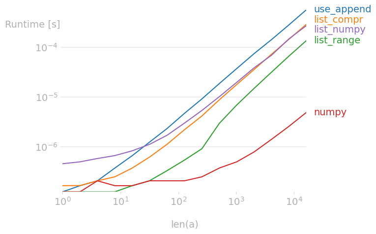
Here's a demo snippet of how it works.
import perfplot
import numpy as np

def use_append(size):
    out = []
    for i in range(size):
        out.append(i)
    return out

def list_compr(size):
    return [i for i in range(size)]

def list_range(size):
    return list(range(size))

perfplot.show(
    setup=lambda n: n,
    kernels=[
        use_append,
        list_compr,
        list_range,
        np.arange,
        lambda n: list(np.arange(n))
    ],
    labels=["use_append", "list_compr", "list_range", "numpy", "list_numpy"],
    n_range=[2**k for k in range(15)],
    xlabel="len(a)",
    equality_check=None
)
Here's what the result chart would look like:
More Advanced
You can also run more elaborate benchmarks with perfplot. In the example below
we're checking the training times for a few scikit-learn pipelines. Pay close
attention to how the generate_data function is used as the setup argument
for perfplot.show.
import perfplot

from sklearn.preprocessing import StandardScaler
from sklearn.pipeline import make_pipeline
from sklearn.datasets import make_regression
from sklearn.linear_model import LinearRegression, Ridge

def generate_data(n):
    # Add a random seed, the video forgot to do this
    X, y = make_regression(n_samples=n)
    return [X, y]

perfplot.show(
    setup=lambda n: generate_data(n),
    kernels=[
        lambda data: LinearRegression().fit(data[0], data[1]),
        lambda data: Ridge().fit(data[0], data[1]),
        lambda data: make_pipeline(StandardScaler(), LinearRegression()).fit(data[0], data[1]),
        lambda data: make_pipeline(StandardScaler(), Ridge()).fit(data[0], data[1]),
    ],
    labels=["lr", "ridge", "std_lr", "std_ridge"],
    n_range=[10**k for k in range(2, 6)],
    xlabel="number of rows in X",
    equality_check=None,
    show_progress=True,
)
This generates a new chart.
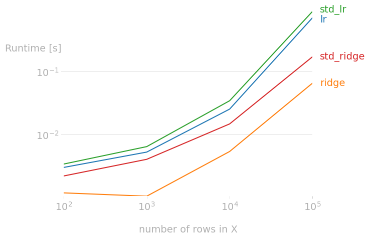
Also note how each function that we're benchmarking is unpacking the data argument.
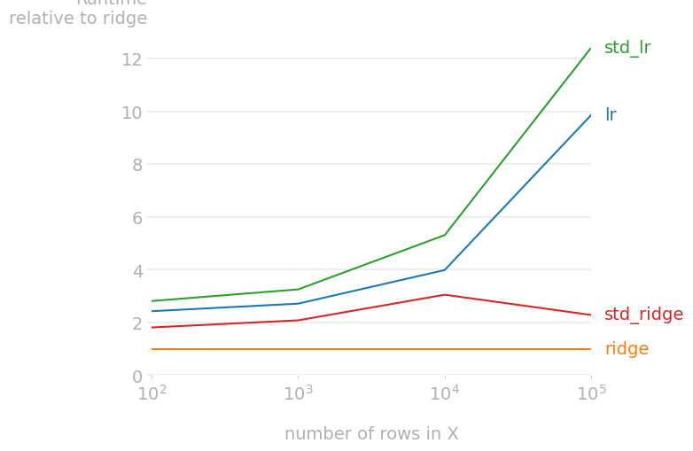
Relative Charts
To make the chart even more explicit, you can also choose to make the chart
relative to one of the implementations. This can be done via the relative_to
argument.
perfplot.show(
    setup=lambda n: generate_data(n),  # or setup=np.random.rand
    kernels=[
        lambda data: LinearRegression().fit(data[0], data[1]),
        lambda data: Ridge().fit(data[0], data[1]),
        lambda data: make_pipeline(StandardScaler(), LinearRegression()).fit(data[0], data[1]),
        lambda data: make_pipeline(StandardScaler(), Ridge()).fit(data[0], data[1]),
    ],
    labels=["lr", "ridge", "std_lr", "std_ridge"],
    n_range=[10**k for k in range(2, 6)],
    xlabel="number of rows in X",
    equality_check=None,
    show_progress=True,
    relative_to=1 # This is the line that's different.
)
Back to main.